Structural Analysis of a Light Aircraft Wing

Executive Summary

Objective: Comprehensive structural integrity assessment and dynamic characterization of a composite light-aircraft wing under aerodynamic loads.
Tools & Methodology: ANSYS Workbench (Fluent, ACP, Mechanical) and Direct Optimization.
Key Achievements: Mapping of 3D CFD pressure fields onto a structural shell/beam model, evaluation of composite failure criteria (Tsai-Wu/Tsai-Hill), and analysis of stress-stiffening effects on modal frequencies.

1. Computational Framework & Composite Setup

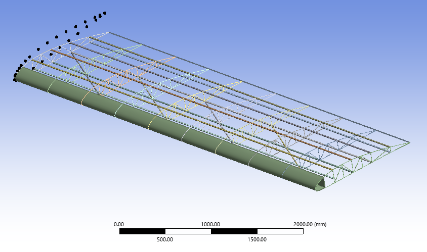
The structural model represents a light aircraft wing (USA35B airfoil) with a span of 10.82 m and a cruise velocity of 48 m/s. The architecture features internal spars, ribs, and stringers modeled as beam elements, with the skin represented by shell elements, as shown in Figure 1.

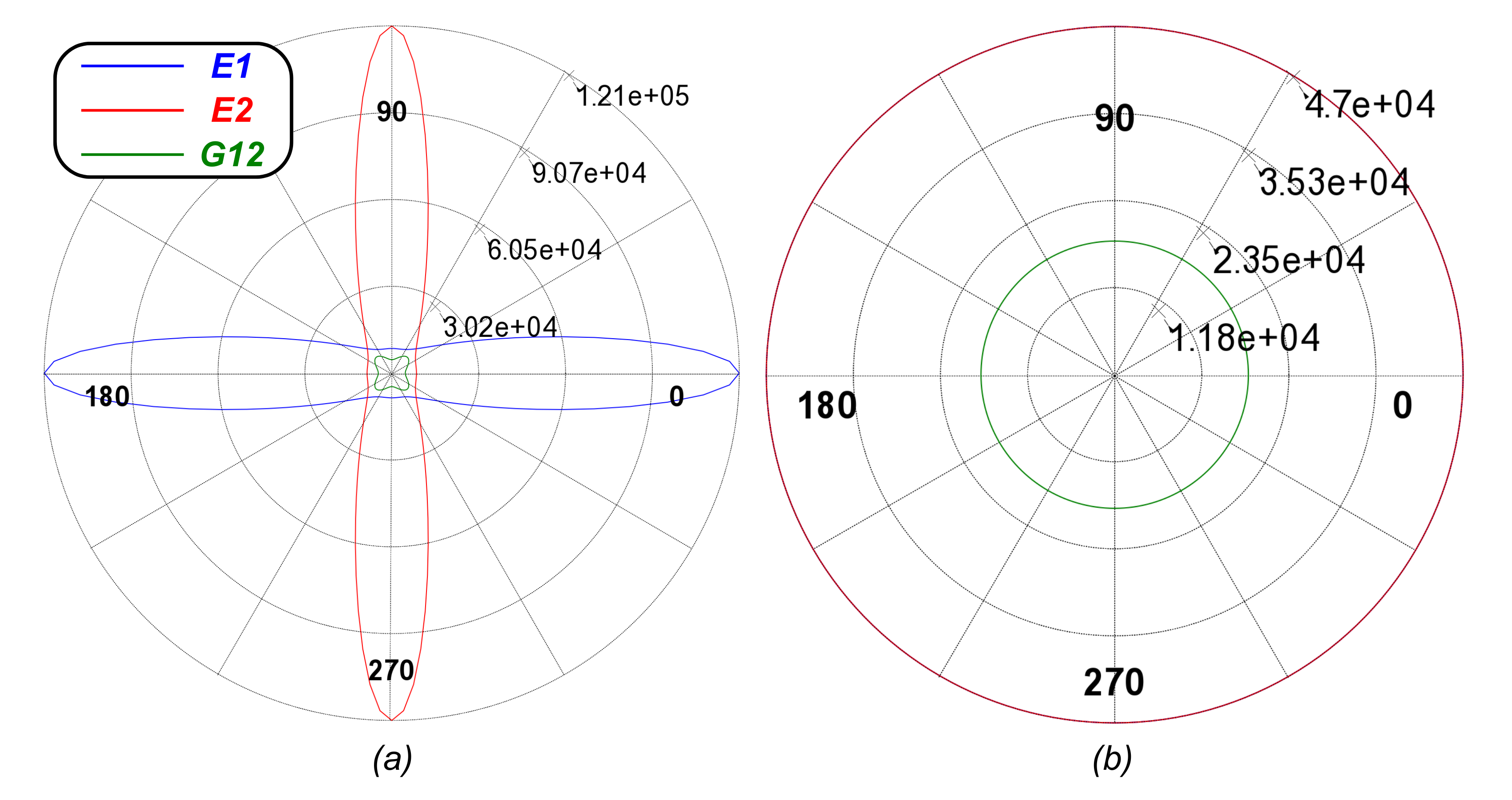
ANSYS Mechanical CAD model showing the internal wing architecture including spars, ribs, and stringers. — **Figure 1** - Internal beam-element architecture of the wing, exposing the structural spar and rib distribution beneath the composite skin.

ANSYS ACP was used to define the anisotropic layup of the carbon fiber skin (symmetric sequence). The resulting polar properties are detailed in Figure 2.

Layup Sequence: [(0/+45/-45/90)_S]₂
Ply Thickness: 0.125 mm

Composite polar properties on ANSYS ACP. — **Figure 2** - Polar properties from ANSYS ACP: (a) ply stiffness, (b) stack-up stiffness.

2. FSI and Static Analysis

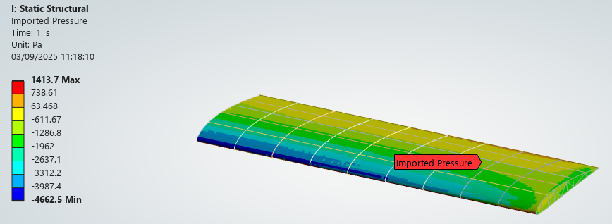
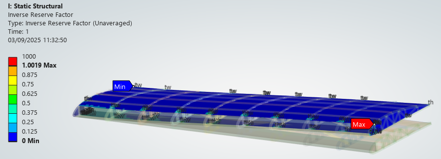
A one-way Fluid-Structure Interaction (FSI) approach was employed. Aerodynamic pressure fields obtained from Fluent (at 10° AoA) were mapped as boundary conditions on the mechanical solver (Figure 3). The resulting structural response was validated against Tsai-Wu and Tsai-Hill failure criteria to ensure integrity under limit load conditions, highlighting critical load-bearing regions as illustrated in Figure 4.

Contour plot of aerodynamic pressure distribution mapped onto the wing surface from a CFD simulation. — **Figure 3** - 3D pressure field imported from ANSYS Fluent mapped directly onto the structural mesh.

Contour plot showing the Inverse Reserve Factor (IRF) on the composite wing, identifying critical stress areas. — **Figure 4** - Composite failure evaluation using Tsai-Wu/Tsai-Hill criteria. The Inverse Reserve Factor (IRF) contour highlights critical load-bearing regions.

3. Parametric Optimization

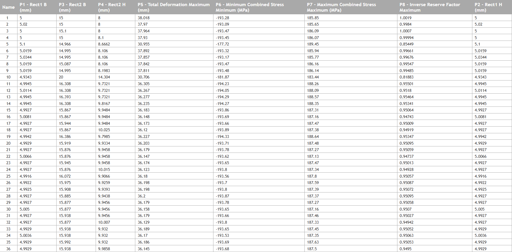
A direct optimization loop was implemented to refine the spar cross-sections, aiming to maximize structural efficiency while maintaining safety margins on composite stress concentrations. The tradeoff results identifying the optimal configuration are represented in Figure 5.

Configuration	Spar 1 Base [mm]	Spar 2 Base [mm]	Max Deformation [mm]	Max Combined Stress [MPa]
Initial	5.00	15.00	38.01	185.85
Optimized	4.99	16.30	36.30	188.26

ANSYS Direct Optimization interface showing the parametric tradeoff results for spar cross-section dimensions. — **Figure 5** - Parametric optimization results identifying the optimal spar dimensions to minimize stress concentrations and weight.

4. Dynamic Characterization

4.1 Pre-Stressed Modal Analysis

To capture realistic flight dynamics, a pre-stressed modal analysis was performed, accounting for the stiffening effect exerted by the aerodynamic lift. The following table compares the natural frequencies before and after the application of the flight load.

Mode	Unstressed Pre-Optimization Frequency [Hz]	Unstressed Post-Optimization Frequency [Hz]	Pre-Stressed Post-Optimization Frequency [Hz]
1	11.76	11.70	11.66
2	43.09	42.63	42.62
3	55.35	55.85	55.86
4	58.60	58.41	58.36
5	77.24	76.70	69.45
6	85.56	86.52	76.68
7	86.48	87.78	78.93
8	87.50	88.35	84.19
9	88.31	89.67	99.95
10	88.73	90.44	102.66
11	91.24	100.13	103.56
12	95.24	100.77	104.43
13	100.69	104.19	109.65
14	101.41	106.06	111.28
15	103.37	111.61	113.27

4.2 Harmonic Response Analysis

A full-method Harmonic Response analysis 10÷60 Hz was conducted to characterize the wing's dynamic behavior, assessing resonant peaks.